Introduction
In short, the Symbolic Aggregate approXimation (SAX) algorithm transforms an input time series into a string.
The algorithm was proposed by Lin et al. and extends the PAA-based approach, inheriting the original algorithm’s simplicity and low computational complexity while providing satisfactory sensitivity and selectivity in range-query processing. Moreover, the use of a symbolic representation opened the door to the existing wealth of data structures and string-processing algorithms in computer science — hashing, regular expressions, pattern matching, suffix trees, and grammatical inference.
The algorithm
SAX transforms a time series X of length n into a string of length \(w\) (where \(w \ll n\), typically), using an alphabet A of size a > 2. The algorithm consists of two steps: (i) it transforms the original time series into the PAA representation, and (ii) it converts the PAA data into a string.
The use of PAA brings the advantage of a simple and efficient dimensionality reduction, while preserving the important lower-bounding property. The actual conversion of PAA coefficients into letters via a lookup table is also computationally efficient, and the contractive property of the symbolic distance was proven by Lin et al.
The discretization from PAA values to symbols is designed so that each symbol occurs with equal probability. This relies on an observation by the algorithm’s original authors: across a large number of examined time series datasets, the values of z-normalized series follow the standard normal distribution N(0,1). Using its properties, it is easy to choose a − 1 breakpoints that slice the area under the Gaussian curve into a equal-probability regions.
Formally, the list of breakpoints \(B = \beta_{1}, \beta_{2}, \ldots, \beta_{a-1}\) such that \(\beta_{i-1} \lt \beta_{i}\), \(\beta_{0}=-\infty\), and \(\beta_{a}=\infty\) divides the area under N(0,1) into a equal areas. By assigning alphabet symbol \(\alpha_{j}\) to each interval \([\beta_{j-1},\beta_{j})\), the vector of PAA coefficients \(\bar{X}\) converts into the string \(\hat{X}\) as follows:
$$ \hat{x}_{i} = \alpha_{j}, \; \text{iff} \; \bar{x}_{i} \in [ \beta_{j-1}, \beta_{j} ) $$SAX also introduces a distance between strings that extends the Euclidean and PAA distances. The function returning the minimal distance between the string representations of two time series \(\hat{Q}\) and \(\hat{C}\) is defined as
$$MINDIST(\hat{Q},\hat{C})\equiv\sqrt{\frac{n}{w}}\sqrt{\sum_{i=1}^{w}(dist(\hat{q}_{i},\hat{c}_{i}))^{2}}$$where the dist function is implemented with a lookup table precomputed for the particular alphabet size, as shown in the table below; the value of each cell (r,c) is computed as
$$ cell_{(r,c)} = \begin{cases} 0, \text{if} \left|r-c \right| \leq 1 \\ \beta_{\max(r,c)-1} - \beta_{\min(r,c)-1}, \text{otherwise}\end{cases}$$The lookup table for the 4-letter alphabet
| a | b | c | d | |
|---|---|---|---|---|
| a | 0 | 0 | 0.67 | 1.34 |
| b | 0 | 0 | 0 | 0.67 |
| c | 0.67 | 0 | 0 | 0 |
| d | 1.34 | 0.67 | 0 | 0 |
As shown by Lin et al., MINDIST lower-bounds the PAA distance applied frame-by-frame, which in turn lower-bounds the Euclidean distance:
$$ \sum_{i=1}^{n}(q_{i}-c_{i})^{2} \;\geq\; \frac{n}{w}\sum_{i=1}^{w}(\bar{q}_{i}-\bar{c}_{i})^{2} \;\geq\; \frac{n}{w}\sum_{i=1}^{w}(dist(\hat{q}_{i},\hat{c}_{i}))^{2} $$The SAX lower bound was examined in great detail by Ding et al. and found superior in precision to spectral decomposition methods on bursty (non-periodic) datasets.
SAX primer
A worked example of the full transform.
1. Time series data
We use the following two time series (their Euclidean distance is 11.42):
> ts1 = c(2.02, 2.33, 2.99, 6.85, 9.20, 8.80, 7.50, 6.00, 5.85, 3.85, 4.85, 3.85, 2.22, 1.45, 1.34)
> ts2 = c(0.50, 1.29, 2.58, 3.83, 3.25, 4.25, 3.83, 5.63, 6.44, 6.25, 8.75, 8.83, 3.25, 0.75, 0.72)
> dist(rbind(ts1, ts2), method = "euclidean")
         ts1
ts2 11.42126
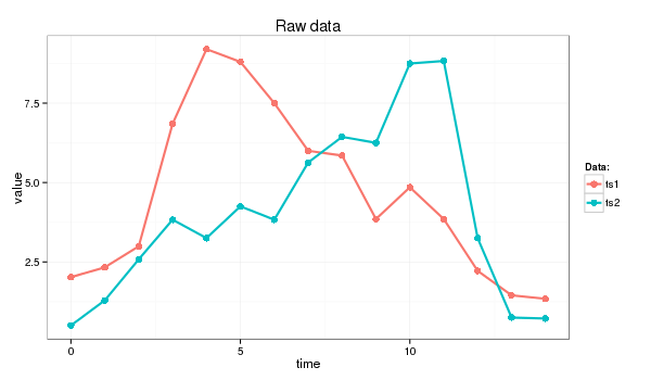
We will transform both into strings of length w = 9 over an alphabet of size a = 4.
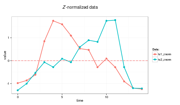
2. Z-normalization
Before applying SAX we z-normalize the data first (see the z-normalization module):
znorm <- function(ts){
  ts.mean <- mean(ts)
  ts.dev <- sd(ts)
  (ts - ts.mean)/ts.dev
}

ts1_znorm = znorm(ts1)
ts2_znorm = znorm(ts2)
See the z-normalization module for the population-\(\sigma\) convention used in the jMotif stack.
3. PAA transform
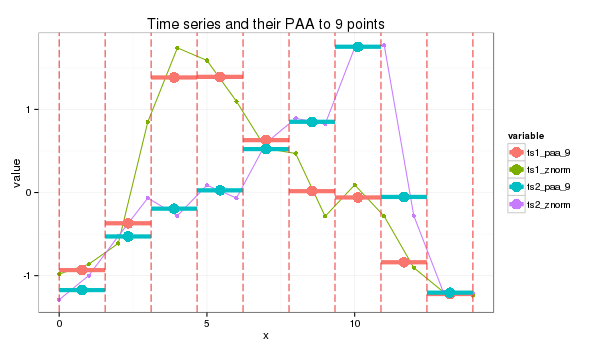
PAA follows the standard procedure:
paa <- function(ts, paa_size){
  len = length(ts)
  if (len == paa_size) {
    ts
  }
  else {
    if (len %% paa_size == 0) {
      colMeans(matrix(ts, nrow=len %/% paa_size, byrow=F))
    }
    else {
      res = rep.int(0, paa_size)
      for (i in c(0:(len * paa_size - 1))) {
        idx = i %/% len + 1 # the frame
        pos = i %/% paa_size + 1 # the point
        res[idx] = res[idx] + ts[pos]
      }
      for (i in c(1:paa_size)) {
        res[i] = res[i] / len
      }
      res
    }
  }
}
paa_size = 9
s1_paa = paa(ts1_znorm, paa_size)
s2_paa = paa(ts2_znorm, paa_size)
4. PAA values to letters
We use the 4-symbol alphabet {a, b, c, d}, as in the lookup table above. The corresponding breakpoints (−0.67, 0, 0.67) are shown as thin blue lines in the plot below.
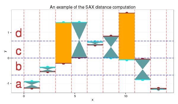
The SAX transform of ts1 through the 9-frame PAA is abddccbaa; the transform of ts2 is abbccddba.
The strings differ in positions 3, 7, and 8, but only two of those differences count: per the lookup table, adjacent letters (such as b and a at position 8) are zero distance apart. Summing the table values position by position gives
and plugging this into the MINDIST definition above yields
$$ MINDIST(\hat{ts1},\hat{ts2}) = \sqrt{\tfrac{15}{9}} \cdot \sqrt{0.67^{2} + 0.67^{2}} \approx 1.22 $$which indeed lower-bounds (very loosely, in this toy example) the true Euclidean distance of 11.42. In the plot, orange marks the symbol pairs whose distance contributes to the total — the letters that are not adjacent in the lookup table.